Markov Decision Process Explained
The basic concepts of Reinforcement Learning

📝This post is part of my personal study notes on Mathematical Foundation of Reinforcement Learning. All diagrams, analogies, tables, and core concepts are drawn from the book. My contribution is the explanation and interpretation in my own words.
Recently, I started learning reinforcement learning as part of a research initiative. The book suggested by my teacher was Mathematical Foundation of Reinforcement Learning by Shiyu Zhao. In this series of explanations, I’ll share my understanding of the book, chapter by chapter.
First things first: What is Reinforcement Learning?
Introduction
Reinforcement learning is the process of teaching an agent to make good decisions on its own. We define the state, the policy (which action to take), the rewards, and the goal, and then let the agent learn from its trajectories and returns as it works toward that goal. This framework is also called a Markov decision process (MDP).
Today, we’ll explore the Markov decision process. But before we get there, we need to make sure the following terms are clear:
State and Action
State Transition
Policy
Reward
Trajectories, Returns, and Episodes
Analogy of Environment
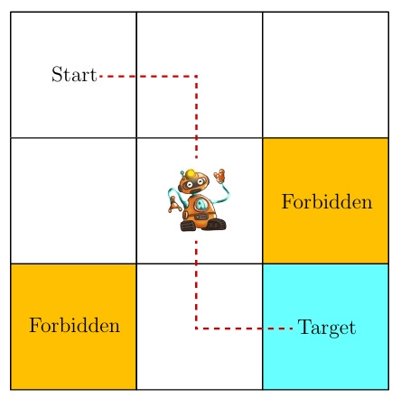
Imagine we have a square grid environment of nine blocks. An agent has been assigned to the grid, with a target of reaching the last cell. In the grid, we have implemented certain conditions:
The agent cannot go out of the boundary of the grid.
There are two forbidden cells that the agent cannot choose.
For our convenience, we will assume the environment is stochastic, with deterministic actions.
Now, let’s start learning the terms of the Markov decision process.
State and Action
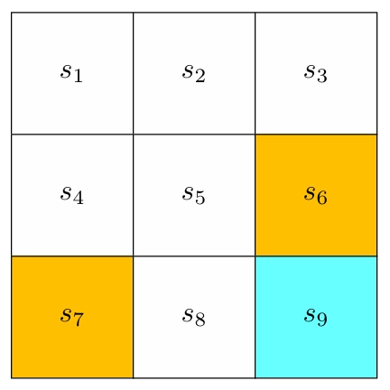
State is the position the agent is placed in compared to its environment. In our environment, we have nine states in the grid. The set of all the states is called the state space, denoted as S = {s1, s2, s3, …, s9}.
We have two types of environments in training:
A stochastic environment, where the output or action is not predetermined and has more than one possibility.
A deterministic environment, where we predetermine the solution and provide it to the agent.
In our case, we will be working with a stochastic environment.
Actions are the possibilities for an agent to move or make decisions. The set of all actions is called the action space, denoted as A = {a1, …….., a5}.
Here in our grid environment, the actions are limited and determined. For example, in a real-life scenario, a strong wind could move our agent from S1 to S8 (or any other state cell), or even throw it out of the boundary. But to make the topic easy to understand, we have eliminated all of these possibilities and predetermined that actions are one cell (state) at a time.
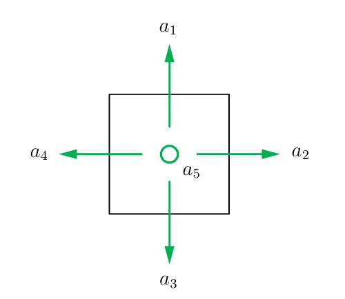
For each state, there are five possible actions:
a1 for moving upward
a2 for moving rightward
a3 for moving downward
a4 for moving leftward
a5 for staying still
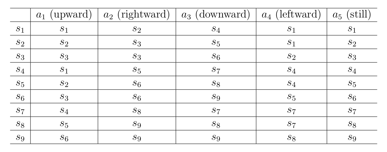
State Transition
State transition is the movement of the agent after taking an action. For example, if the agent moves from s1 to s2, the state transition would be:
In our environment, there are two scenarios:
Scenario 1: The agent tries to get out of the boundary but is bounced back because it is not accessible.
\(s_1 \xrightarrow{a_1} s_1\)Scenario 2: The agent tries to enter the forbidden cell. If it is not accessible, it will not be able to enter.
\(s_5 \xrightarrow{a_2} s_5\)But in our case, the agent can access the forbidden cell, and the agent may get punished for entering it. More about the punishment is in the reward section.
\(s_5 \xrightarrow{a_2} s_6\)
In real-world applications, the state transition process is determined by real-world dynamics.
Here is a table of the state transition process in a deterministic state transition. Each cell indicates the next state to transition to after the agent takes an action at a state.
Probability theory is necessary for studying reinforcement learning, so readers are advised to get familiar with it.
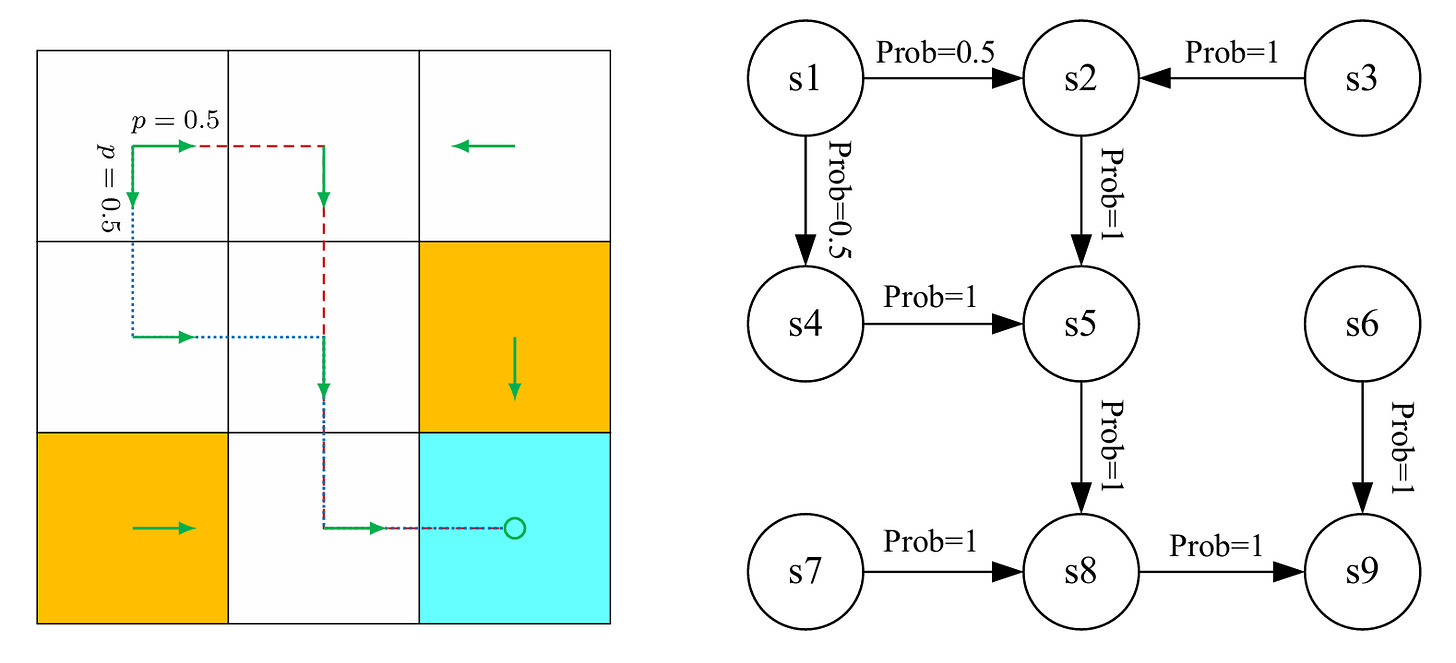
We can explain the state transition process mathematically by using conditional probability. For example, to go from s1 to a different cell using a2, the conditional distribution would be:
In our grid, if we look into it, we will see that only s2 can be accessed from s1 by using a2. That is why the probability of getting to the S2 cell is 1, and the rest are 0.
Policy
Policy is the guidance the agent uses to choose its actions. We can use arrows to illustrate a policy in our grid.
Just like our environment, policies can also be deterministic and stochastic. In the deterministic policy, the trajectories of the agent are one-way or fixed. As we can see in the figure below, the arrows of trajectories are fixed in one way.
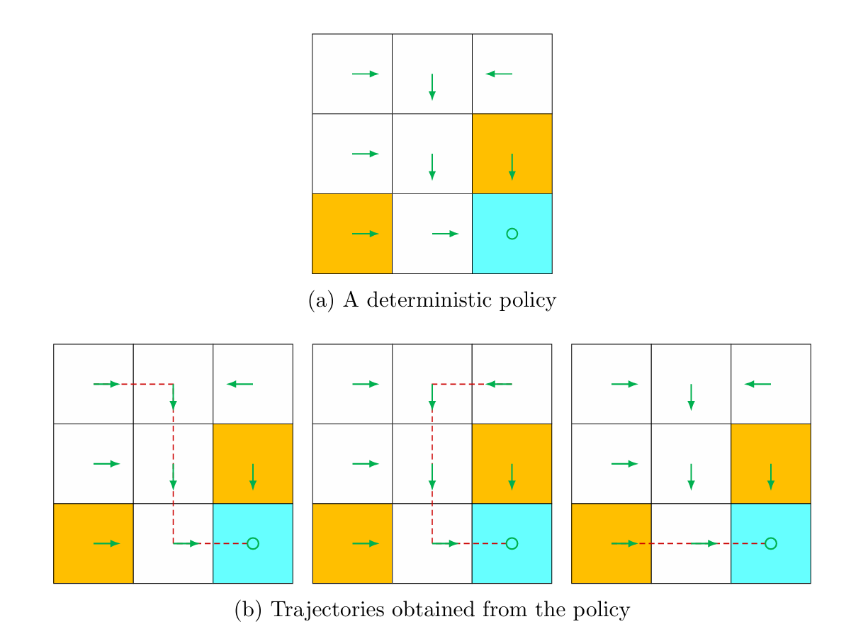
Policy can also be expressed mathematically with conditional probability. Let’s say, we denote policy as π(a|s), then the conditional distribution function defined for s1 in deterministic policy is,
Policy can also be stochastic in general. Normally, in an environment, there can be multiple policies for an agent to move. For example, in the figure below, we can see from state s1 that the agent can take two different actions, rightward or downward.
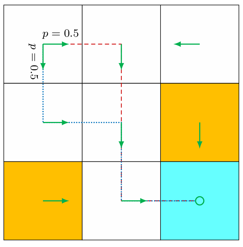
In this case, these two actions have the same probability: p = 0.5.
Here is a table of the stochastic policy. Each entry indicates the probability of taking an action at a state.
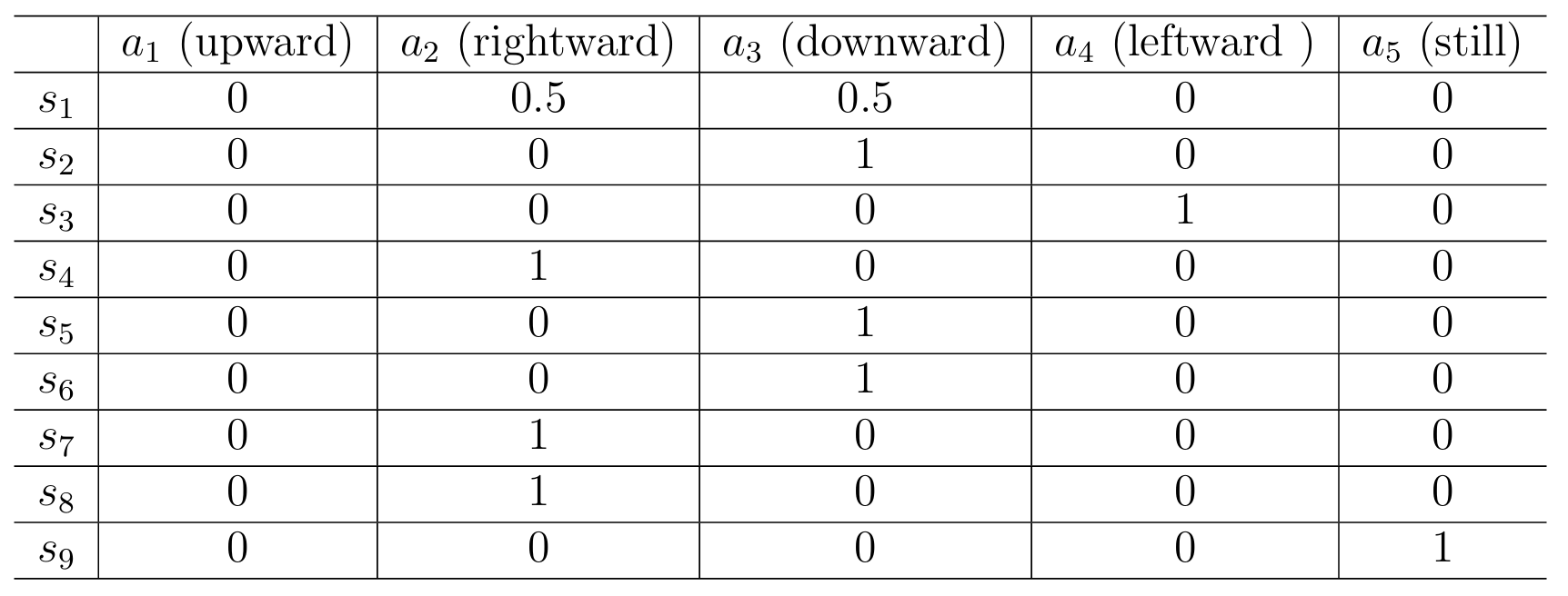
A tubular representation shows the entry in the ith row and jth column as the probability of taking the jth action in the ith state.
Reward
A reward, true to its name, is a prize to the agent to let it know which action is best to take. A reward can be viewed as a human-machine interface that we can use to guide the agent to behave as we expect. In reinforcement learning, it is an important step to design proper rewards.
We can denote the reward as r(s, a). The values of a reward can be positive or negative, or a real number or zero. Basically, with a positive reward, we motivate the agent to take the corresponding action. With a negative reward, we discourage the agent from taking that action. Negative reward can also be depicted as punishment for the agent.
For example, in our grid world, the rewards are designed as follows:
We need to calculate the total reward to determine a good policy. A simpler approach is to use conditional probabilities p(r | s, a) to describe the reward process.
Trajectories, Returns, and Episodes
A trajectory is the sequence of states, actions, and rewards the agent experiences. Trajectories are also known as a state-action-reward chain.
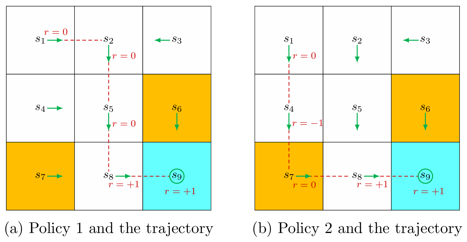
For example, the trajectories of Policy 1 in the figure would be:
The Returns are total rewards or cumulative rewards. Returns can be used to evaluate policies. For example, the return of the trajectory of Policy 1 is,
Returns are a combination of immediate rewards and future rewards. Immediate reward is the reward that the agent gets after taking an action at the initial state, and the future reward is what the agent gets after leaving the initial state.
There is a possibility that initially the immediate reward is negative, but the future reward is positive, which makes the return of the policy to zero or a positive real number.
For example, in Policy 2, the trajectories are,
Here, the return of the trajectories is:
So we can say from the result that the policy and the trajectories in Policy 1 would be the best route to take for our agent.
Thus, which actions to take should be determined by the return (i.e., the total reward) rather than the immediate reward to avoid short-sighted decisions.
There is another type of return in reinforcement learning, called discounted returns. Remember, we have discussed the action of staying still in a position? We defined that action as a5. We can design a policy where the agent will stay at the state 9 (s9) for infinite time. Or maybe the agent can choose to stay at that position because the agent is getting rewards of +1 by staying there. In this case, the trajectory would be:
The return of this trajectory would be:
As we can see, the sequence of returns does not settle to a finite value. Therefore, we need to learn about the discounted return for such long trajectories.
A discounted return is basically the sum of the discounted rewards, which is used to get infinite trajectories. For example, in the infinite trajectories above, the discounted returns would be,
where,
γ ∈ (0,1) is called the discount rate.
When γ is close to 0, then the agent looks for the near future for +1 (prioritizes immediate rewards).
When γ is close to 1, then the agent looks into the far future for more +1 (values future rewards more).
When the reward +1 is far away, only then does the agent dare to go for the negative rewards (-1).
There might be some points where the agent pauses while following a policy. If an agent stops at a certain point while following a policy, those certain stops are called terminal state, and the trajectory it takes because of this state is called an episode/trial.
The status of an episode can vary depending on the environment. For example,
If the policy is deterministic, we will get the same episode every time.
But if the policy or the environment is stochastic, we may get a different episode.
An episode is usually assumed to be a finite trajectory. While completing a task, if there are episodes, then they are called episodic tasks. However, there may be some tasks with no terminal states, meaning the task will continue infinitely; such tasks are called continuing tasks.
We can convert episodic tasks to continuous ones in unified mathematical terms. The agent can continue taking actions in two ways to convert/unify the episodic and continuous tasks:
Treat the terminal state as a special state and define or fix its action, such as A(s9) = {a5}, so it will continue to stay there forever.
Treat the terminal as a normal state, it will find its way and learn to stay or come back at s9 as it is giving it a reward every time it comes back.
Markov Decision Processes
A Markov decision processes (MDP) is a general framework for describing stochastic dynamical system.
The key ingredients of an MDP are listed below:
Sets:
State space: the set of all states, denoted as S.
Action space: a set of actions, denoted as A(s), when each state is defined as s ∈ S.
Reward Set: a set of rewards, denoted as R(s, a), associated with each state-action pair (s, a).
Model:
State Transition Probability: In state s, when taking action a, the probability of transitioning to state s is p(s’ | s, a). The state transition probability follows,
\(\begin{equation*} \sum_{s' \in \mathcal{S}} p(s' \mid s, a) = 1 \text{ for any } (s, a) \end{equation*} \)Sum of p of s‑prime given s and a equals one. Simply put, if we are in state s, and we take action a, we must end up somewhere. So all the chances of going to each possible next state must add up to 1.
Reward probability: In state s, when taking action a, the probability of obtaining reward r is p(r | s, a). The reward probability follows,
\(\begin{equation*} \sum_{r \in \mathcal{R}} p(r \mid s, a) = 1 \text{ for any } (s, a) \end{equation*} \)For every state–action pair (s, a), the probabilities of all possible rewards r that can occur when taking action a in state s form a valid probability distribution. Meaning, if we are in state s and take action a, we must get some reward. So all the chances of getting each possible reward must add up to 1.
Policy:
In state s, the probability of choosing action a is π(a | s). For any s ∈ S it holds that,
\(\begin{equation*} \sum_{a \in A(s)} \pi(a \mid s) = 1 \end{equation*} \)Markov Property:
The Markov property refers to the memoryless property of a stochastic process. Mathematically, it means that,
\(\begin{equation*} p(s_{t+1} \mid s_t, a_t, s_{t-1}, a_{t-1}, \ldots, s_0, a_0) = p(s_{t+1} \mid s_t, a_t) \end{equation*} \)\(\begin{equation*} p(r_{t+1} \mid s_t, a_t, s_{t-1}, a_{t-1}, \ldots, s_0, a_0) = p(r_{t+1} \mid s_t, a_t) \end{equation*}\)where t represents the current time step and t + 1 represents the next time step.
The equation indicates that the next state or reward depends merely on the current state and action, and is independent of the previous one. The Markov property is important for deriving the fundamental Bellman equation of MDPs.
Here, in the Markov decision process, for all (s, a)I,
- p(s’ | s, a) is called model.
- p(r | s , a) is called dynamics.
A model can be stationary or non-stationary. A stationary model does not change over time, but a non-stationary model may change over time.
Markov Processes (MPs):
There can be confusion between Markov Processes (MPs) and Markov decision processes (MDP). The difference between MP and MDP is that, once the policy of an MDP is fixed, the MDP transforms into an MP.
For example, in the grid world example, it can be defined as a Markov process. (MP). If the number of states is finite or countable and it is a discrete-time process, then the Markov process can also be called a Markov chain.
Markov Processes or Markov Chain In our series of explanations, we will use finite MDPs.

Conclusion
“Finally, reinforcement learning can be described as an agent-environment interaction process. The agent is a decision-maker that can sense its state, maintain policies, and execute actions. Everything outside of the agent is regarded as the environment. In the grid world examples, the agent and environment correspond to the robot and grid world, respectively. After the agent decides to take an action, the actuator executes such a decision. Then, the state of the agent would be changed and a reward can be obtained. By using interpreters, the agent can interpret the new state and the reward. Thus, a closed loop can be formed.”